The aim of this section is to explain a fundamental problem in economics, the derivation of a consumer’s demand function, in a very simple way. The article is organized as follows:
- Conceptual review of assumptions in demand theory
- Description of the Utility Maximization Problem
- Derivation of the Expenditure Minimization Problem
Assumptions
The consumer theory assumes that the consumer is rational. This implies that his preferences satisfy the following properties: 1. They are complete; that is, given any set of possible bundles of goods, the consumer is always capable of deciding which one is preferable to the others and then ranking them in terms of preference.2. They are reflexive; it means that any bundle is at least as good as itself.
3. They are transitive; meaning that if a bundle
 is preferred to a bundle
  , and this bundle is preferable to a third bundle
  , then it is implied that the first bundle will be preferred to the bundle .
4. They are continuous; there are no big jumps in the ranking of alternatives.
The fulfillment of these properties ensures that consumer’s preferences are consistent and can be represented by an utility function,
 such that if bundle is preferred to bundle , then
The locus of all bundles that give a certain level of utility to the consumer constitutes an indifference curve (or level curve), which is the usual way of representing preferences. Nevertheless, in spite of these four properties, there is still the possibility of having “special cases” such as the existence of perfect substitutes or perfect complements, among others, which lead to special shapes for the indifference curves. For avoiding these cases, two additional properties are assumed:
5. Preferences are monotonic, or “more is preferred to less”; this implies that, given any set of two bundles, if one of them contains at least as much of all goods and more of one good than the other, then the first bundle will be preferred to the second.
6. Preferences are convex; that is, any combination of two equally preferable bundles will be more desirable than these bundles.
These five properties confer a special shape to level curves: they are downward slopping and convex.
Utility Maximization Problem
This section develops the Utility Maximization Problem (UMP) for the simplest case of only two goods. The model can easily be generalized to goods.
Assume that there are two goods,
 and
and  , whose prices are
  and
and  , respectively. The consumer has a fixed amount of income,
  , for spending on consumption, and his preferences are represented by a generic utility function,
  , with
  ,
,  .
The consumer’s aim is to obtain the maximum possible utility but he is
constrained by his level of income. He cannot spend more than , thus he faces a budget constraint:
.
The consumer’s aim is to obtain the maximum possible utility but he is
constrained by his level of income. He cannot spend more than , thus he faces a budget constraint:  1
1Formally, the problem can be formulated as follows:
Max
subject to And it can be solved by the Lagrange Multipliers method:
Max


The first order conditions (FOC) are:

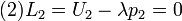

Note that conditions
 and
and  imply that
  .
That is, the marginal rate of substitution (MRS) must be equal to the
relation of prices, and it means that the indifference curve must be
tangent to the budget constraint.
.
That is, the marginal rate of substitution (MRS) must be equal to the
relation of prices, and it means that the indifference curve must be
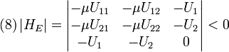
tangent to the budget constraint.The second order conditions (SOC) are:

It can be demonstrated that the SOC imply that indifference curves are convex. The reciprocal is true only for the case of two goods.
The solutions to the FOC are
 ,
, ,
, .They depend on prices and income, thus they can be written as
  ,
, ,
, .The functions and ,< are the Marshallian Demand Functions. They represent the amount of goods and , that the consumer is willing to purchase given their prices, income and tastes.
Another concept that emerges from the UMP is the Indirect Utility Function, and it can be obtained by replacing the Marshallian demands into the utility function. By definition, it also is a function of prices and income, then it can be written as
 . Intuitively, it represents the maximum utility that the consumer can achieve for any given values of
  .
.Note that, because of the Envelop Theorem, it must be the case that
 .
It implies that the Lagrange multiplier can be thought as the marginal
utility of income. That is, it represents the rate of change of the
maximum utility that is derived from an infinitesimal rise in income.
.
It implies that the Lagrange multiplier can be thought as the marginal
utility of income. That is, it represents the rate of change of the
maximum utility that is derived from an infinitesimal rise in income.1 Striclty, the constraint is
 , but the monotonicity assumption ensures that he will spend all his income.
Expenditure Minimization Problem
The Expenditure Minimization Problem (EPM) is the dual problem of the UMP and it can be thought as follows. Consider a consumer who gets utility through the consumption of the two goods. In this case, there is no restriction on the income to be spent, but the consumer must be on a certain level curve, .
Given this constraint, his objective is to reach this indifference
curve with the minimum possible expenditure. Therefore, the problem is:
.
Given this constraint, his objective is to reach this indifference
curve with the minimum possible expenditure. Therefore, the problem is:Min
 subject to
Again, this constrained optimization can be solved by the Lagrange Multipliers method:
Min


The FOC of this program are:


And the SOC are:
Note that conditions
 and
and  imply the same tangency condition than the UMP: . In this program, it means that the expenditure function must be tangent to the indifference curve .
Solving equations
to  gives the optimal levels of
  ,
, ,
, .The demand functions and
  are the Hicksian (or Compensated) Demand Functions. Note that these demands depend on prices and the utility level, therefore they are denoted
  ,
, ,
, .
.The function resulting from replacing the Hicksian demands into the expenditure function gives the minimum expenditure necessary to reach
for any given values of  . It is called the Indirect Expenditure Function and is denoted
  .
.Again, the Lagrange multiplier has a special interpretation. The Envelop Theorem implies that
 ,
meaning that the Lagrange multiplier represents the rate of change of
the expenditure function given a change in the utility level to reach.
,
meaning that the Lagrange multiplier represents the rate of change of
the expenditure function given a change in the utility level to reach.
No comments:
Post a Comment